Title: DBS101 Unit 6

categories: [DBS101, Unit 6] tags: [DBS101]

Topic: Database Indexing, Query Processing, and Optimization

Introduction

Before learning about Unit 6, I thought databases just stored data and we could get it back with simple queries. I didnt know there was so much happening behind the scenes! I knew SQL commands like SELECT and JOIN, but I had no idea about how the database actually finds and processes the data. After going through Unit 6, I now understand that databases use special structures called indexes to make searching faster, and there’s a whole process for handling and optimizing queries efficiently. What really surprised me was learning about B+ trees and how they organize data for quick access, and how query optimization can make a huge difference in performance. The exercises we did in class where we created indexes and analyzed query plans helped me see the real-world impact of these concepts. It’s like learning the difference between knowing how to drive a car and actually understanding how the engine works!

Important Lessons from Unit 6

Understanding Indexes in Databases (Lesson 14)

The first major topic we learned was about database indexes. Indexes are special lookup tables that help the database find data faster. They’re kinda like the index at the back of a book that helps you find information quickly without reading the whole book.

Without indexes, the database would have to scan every single row in a table to find the data you’re looking for. This would be super slow for large databases! As our teacher explained, “Indices are critical for efficient processing of queries in databases. Without indices, every query would end up reading the entire contents of every relation that it uses.”

There are two main types of indexes:

1. Ordered Indices: These store values in a sorted order.
2. Hashed Indices: These distribute values across buckets using a hash function.

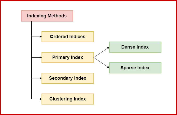
Ordered Indices

Ordered indices store search key values in sorted order and link each search key with the records that contain it. Based on how records are stored, there are two types:

• Clustering Index (Primary Index): The records in the file are stored in the same sorted order as the index entries. Each index entry has a search key value and a pointer to the first record with that key.
• Non-clustering Index (Secondary Index): The records in the file are not sorted in the same order as the index entries. Each index entry has a search key value and pointers to all records with that key.

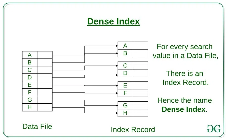
We also learned about dense and sparse indexes:

• Dense Index: An index entry exists for every search-key value in the file.
• Sparse Index: An index entry exists for only some of the search-key values, and the file must be sorted by the search key.

Here’s an example of creating a dense index in PostgreSQL:

CREATE INDEX employees_idx ON employees (emp_id);

This creates a dense index where each index entry contains the “emp_id” value and a pointer to the matching record in the “employees” table.

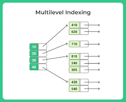
Multilevel Indexing

When indexes get too big to fit in memory, we use multilevel indexing. This is like having an index on the index itself! It consists of:

• The main index (inner index) stored on disk
• A smaller outer index that contains some entries from the inner index and can fit in memory

This approach reduces the number of disk accesses needed to find a record, making searches much faster.

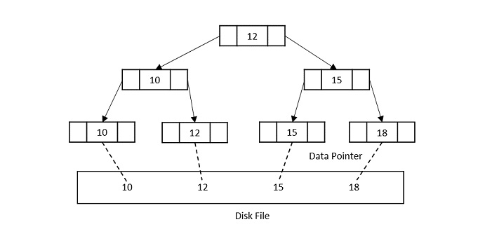
B+ Trees

The most important indexing structure we learned about was the B+ tree. B+ trees are used a lot because they stay efficient even when data is added or deleted.

A B+ tree is a balanced tree where every path from the root to a leaf has the same length. Each non-leaf node has between ⌈n/2⌉ and n children, where n is fixed for a particular tree.

The key things about B+ trees:

• They are perfectly balanced (every leaf node is at the same depth)
• Every node except the root is at least half-full
• Inner nodes only guide the search, while leaf nodes store the actual values

We also learned about the difference between B-trees and B+ trees:

• In a B-tree, keys and values are stored in all nodes
• In a B+ tree, values are only stored in leaf nodes, and inner nodes only guide the search

This makes B+ trees better for disk-based storage because inner nodes can store more keys, making the tree shorter and reducing disk accesses.

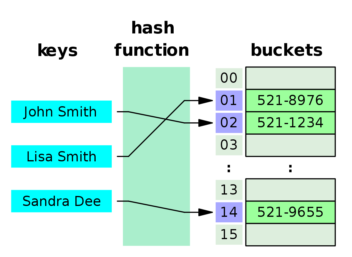
Hash Indices

Hash indices use a hash function to map search keys to bucket addresses. They’re very good for equality searches but don’t work for range queries.

The basic process works like this:

1. To insert a record with key Ki, compute h(Ki) to get the bucket address
2. Add the record entry to that bucket
3. For lookups, compute the hash function and go directly to the bucket

Hash indices are great for exact matches but can’t handle range queries like “find all employees with salary between $50,000 and $70,000.”

Query Processing (Lesson 15)

The second major topic we covered was query processing, which means all the activities involved in getting data from a database. This includes translating high-level queries (like SQL) into expressions that the database can use, optimizing these expressions, and evaluating them.

Steps in Query Processing

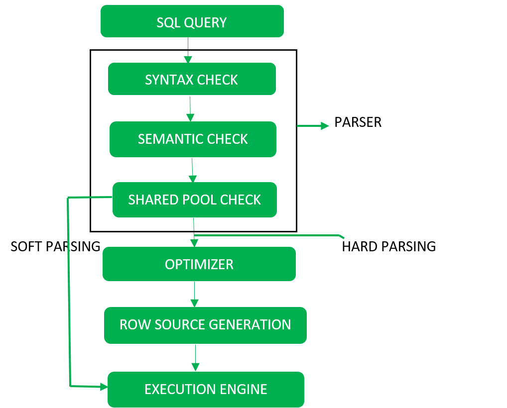
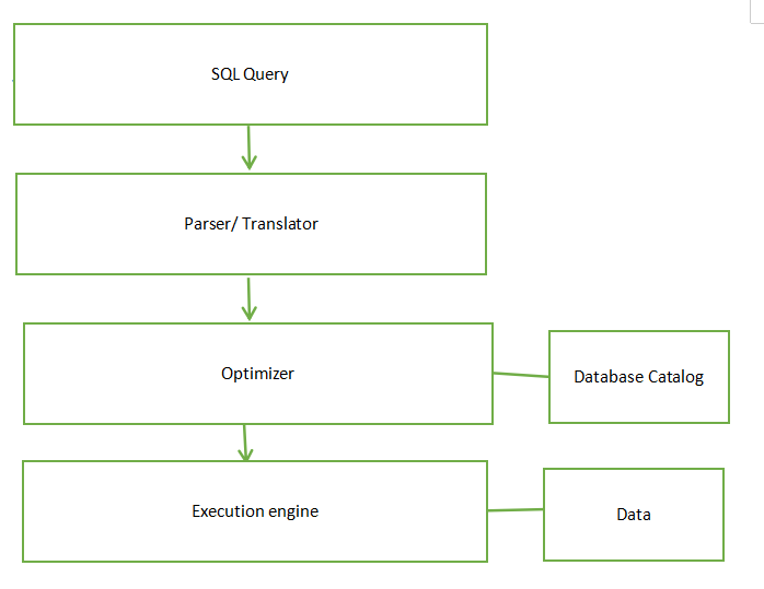
There are three main steps in query processing:

1. Parsing and Translation: Queries written in high-level languages like SQL are translated into an internal form based on relational algebra. This involves checking syntax, validating relations, parsing into a tree, and translating into a relational algebra expression.
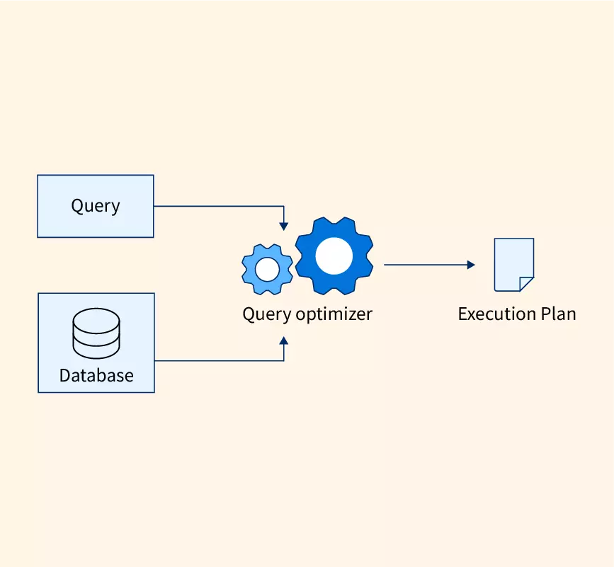
2. Optimization: The query optimizer chooses the most efficient way to execute the query by estimating the cost of different plans and selecting the one with the lowest cost.
3. Evaluation: The query execution engine takes the optimized plan and executes it to produce the result.

Query Evaluation

SQL is a declarative language, which means it says what data to get but not how to get it. The database system converts SQL queries to relational algebra, which specifies the exact steps to execute.

A query evaluation plan is a sequence of operations that can be used to evaluate a query. It’s typically shown as a tree where each node is an operation (like selection, projection, or join) and the edges show the flow of data.

Measures of Query Cost

We learned that traditionally, query cost was calculated based on I/O access to data, especially when working with large databases on magnetic disks. The cost formula was:

Cost = b * tT + S * tS

Where:

• b is the number of blocks transferred
• S is the number of random I/O accesses
• tT is the average block transfer time
• tS is the average block access time (disk seek time + rotational latency)

However, with modern storage devices like SSDs and in-memory databases, I/O costs have less impact, and CPU costs become more important. But since CPU costs are hard to calculate, we focused on I/O costs in our class.

Query Execution Methods

We learned about two main approaches for executing queries:

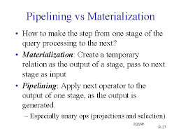
1. Materialization: Store intermediate results in temporary relations. This involves:

2. Evaluating lowest-level operations
3. Storing results in temporary relations

4. Using these results for higher-level operations

5. Pipelining: Pass results directly from one operation to the next without creating temporary relations. This:

6. Reduces cost by eliminating temporary relations
7. Can start generating results early
8. Uses an iterator interface with open(), get_next(), and close() methods

Database Operations and Their Costs

We also learned about various database operations and how to evaluate their costs:

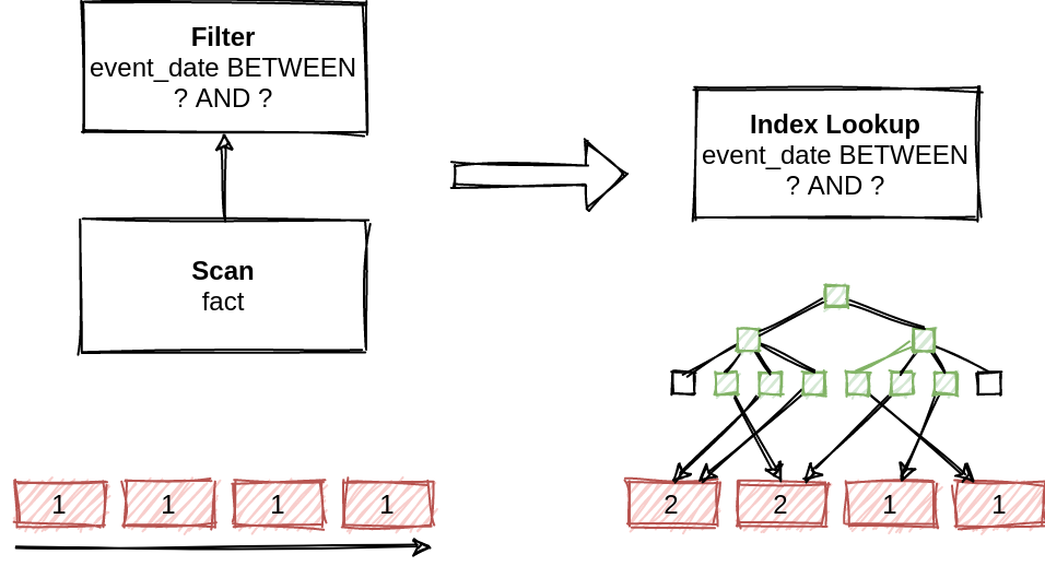
• Selection Operation: Retrieving records that satisfy certain conditions using linear search, binary search, or index-based selection.
• Sorting Operation: Using external sort-merge algorithm when data is too large to fit in memory.
• Join Operation: Using nested-loop join, block nested-loop join, indexed nested-loop join, or merge join.
• Other Operations: Including duplicate elimination, projection, set operations, outer join, and aggregation.

Query Optimization (Lesson 16)

The third major topic was query optimization, which is the process of selecting the most efficient query-evaluation plan from among the many strategies possible for processing a given query.

Transformation of Relational Expressions

Relational algebra expressions can be transformed into equivalent expressions with different evaluation costs. Two expressions are equivalent if they generate the same set of tuples on every legal database instance.

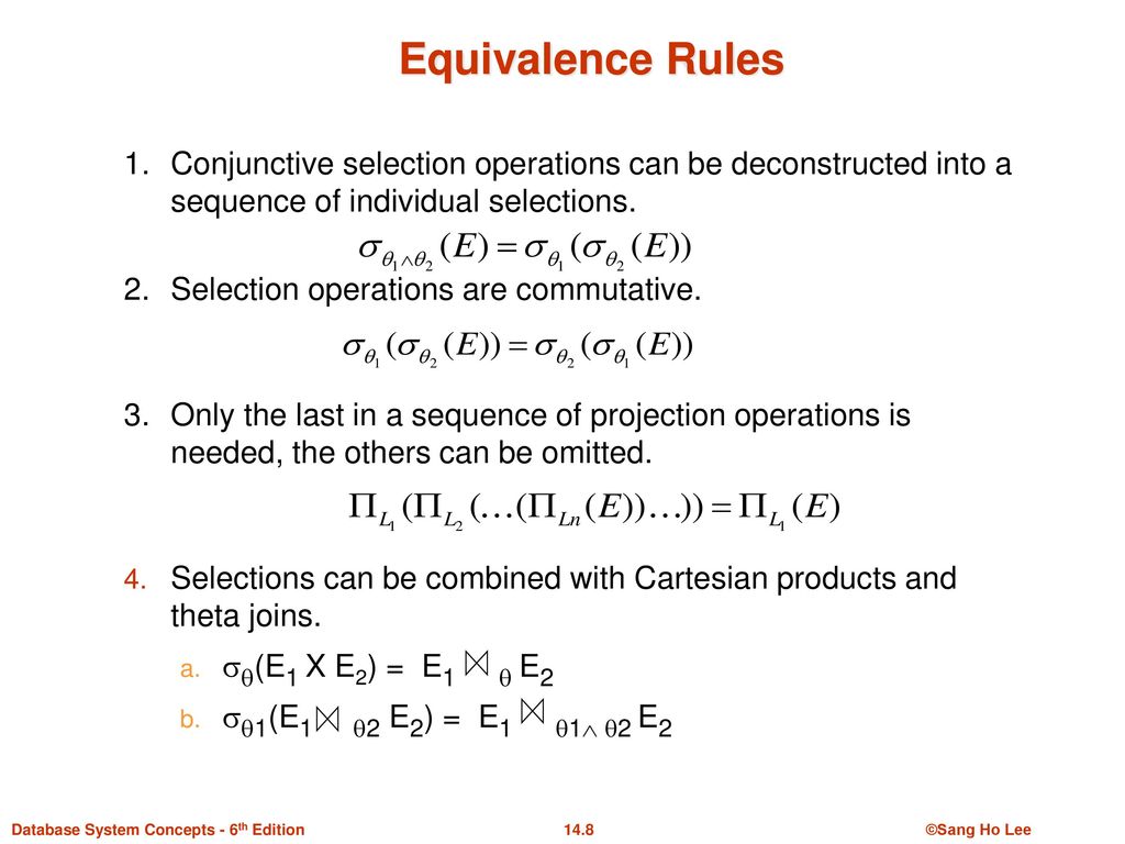
Query optimizers use equivalence rules to transform expressions into more efficient forms. Some important equivalence rules include:

• Conjunctive selection can be deconstructed: σθ1∧θ2(E) ≡ σθ1(σθ2(E))
• Selection operations are commutative: σθ1(σθ2(E)) ≡ σθ2(σθ1(E))
• Theta joins are commutative: E1 ⋈θ E2 ≡ E2 ⋈θ E1
• Natural joins are associative: (E1 ⋈ E2) ⋈ E3 ≡ E1 ⋈ (E2 ⋈ E3)
• Selection distributes over join: σθ1(E1 ⋈θ E2) ≡ (σθ1(E1)) ⋈θ E2 (if θ1 only involves E1)

Join Ordering

Join ordering is important for reducing intermediate result sizes. Since natural joins are associative and commutative, we can reorder them to minimize the size of intermediate results.

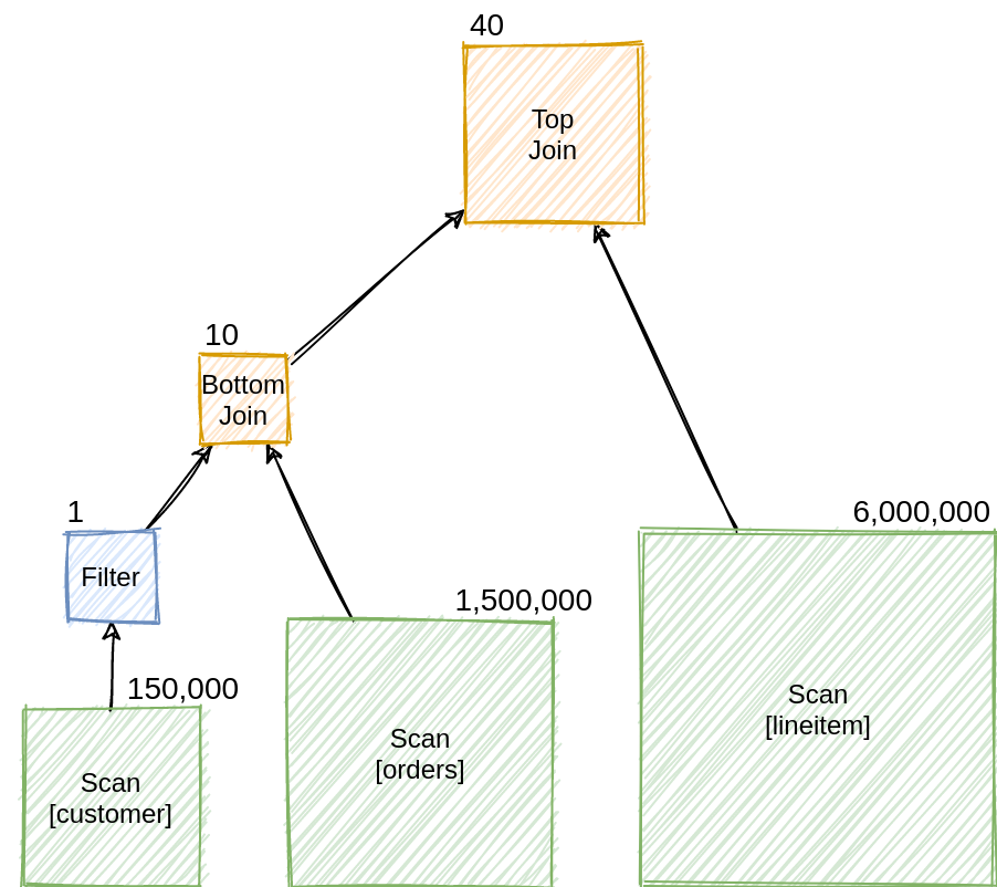
For example, consider the query:

SELECT * FROM customer, orders, lineitem
WHERE customer.c_custkey = orders.o_custkey
AND orders.o_orderkey = lineitem.l_orderkey
AND customer.c_mktsegment = 'BUILDING'

There are two possible join orders:

1. (σc_mktsegment=’BUILDING’(customer) ⋈ orders) ⋈ lineitem
2. (orders ⋈ lineitem) ⋈ σc_mktsegment=’BUILDING’(customer)

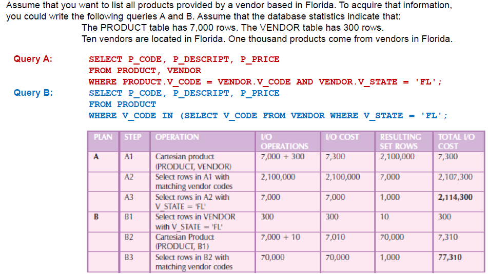
The first join order is more efficient because it filters customers early, resulting in a smaller intermediate relation. The second join order produces a large intermediate relation because it joins orders and lineitem first, only to discard most of the tuples in the second join.

Cost-Based Optimization

Query optimizers use cost-based optimization to choose the best execution plan. This involves:

• Exploring the space of all equivalent query evaluation plans
• Using equivalence rules to generate alternative plans
• Choosing the plan with the least estimated cost

The optimizer considers both join order selection and choosing join algorithms (nested loop, hash join, etc.).

For example, for the query:

SELECT * FROM R, S, T WHERE R.A = S.B AND T.C = S.D

Alternative plans by join order could be:

1. (R JOIN S) JOIN T
2. (S JOIN T) JOIN R
3. (R JOIN T) JOIN S

The optimizer would estimate the cost of each plan and choose the one with the lowest cost.

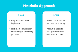
Optimization Heuristics

To reduce the cost of optimization itself, query optimizers use heuristics such as:

• Perform selections early to reduce data size
• Perform projections early after selections
• Use left-deep join trees (easy for pipelining)
• Cache plans for repeated queries with different constants

For example, for the query:

SELECT * FROM R, S, T WHERE R.A = S.B AND S.C = T.D AND R.E > 10

A heuristic plan might be:

1. Scan R, apply filter R.E > 10
2. Index nested loop join with S using R.A = S.B
3. Index nested loop join with T using S.C = T.D

Nested Subqueries

Correlated evaluation (invoking a subquery repeatedly) is very inefficient. Query optimizers try to decorrelate nested subqueries by rewriting them using joins, semijoins, or anti-joins.

For example, the query:

SELECT name FROM instructor 
WHERE exists (SELECT * FROM teaches WHERE instructor.ID = teaches.ID AND teaches.year = 2019)

Can be rewritten using a semijoin as:

Πname(instructor ⋉instructor.ID=teaches.ID ∧ teaches.year=2019 teaches)

My Experience and Reflections

At first, I found indexing really confusing. There were so many types and terms like “clustering” and “non-clustering” that I kept mixing up. During one lab session, I created a index on the wrong column and couldnt figure out why my queries werent getting faster! It took me like 20 minutes to realize my mistake.

B+ trees were super hard to get. I kept getting confused about the diference between B-trees and B+ trees. But after our teacher drew it on the board and showed us how the search works step by step, it started to make sense. I still struggle with remembering all the propertys tho, like how many keys each node can have and stuff.

Query processing was easier to understand cuz its more logical - you parse the query, optimize it, and then execute it. But the cost calculations were tricky. I kept forgeting the formula and mixing up the variables. And when we had to calculate the cost of different join algorithms, I got totally lost trying to figure out which one would be more efficient in different situations.

The most intresting part for me was learning about query optimization and how changing the order of joins can make such a big difference in performance. In one lab, we ran the same query with different join orders, and the difference was huge! One version took like 15 seconds, but the optimized version ran in less than a second. That really showed me why this stuff matters in real life.

I still have trouble with some of the equivalence rules for transforming relational expressions. There are so many of them, and I cant remember which ones to apply in which situations. During our group project, I spent hours trying to optimize a complex query, but I kept making mistakes in applying the rules. Eventually my friend helped me figure it out.

The pipelining concept was also confusing at first. I didnt understand how results could be passed from one operation to another without storing them somewhere. But the iterator interface with open(), get_next(), and close() methods made it clearer. Its like how water flows through pipes without needing to be stored in tanks along the way.

Overall, Unit 6 was probably the hardest unit so far, but also the most useful for understanding how databases actually work behind the scenes.

Conclusion

Unit 6 has really opened my eyes to whats happening behind the scenes in databases. I now understand that its not just about writing correct SQL queries, but also about making them run fast by using indexes and optimizing query plans.

The most valuable thing I learned was definately about indexes and how they can make queries run way faster. I also now understand why query optimization is so important - a good query plan can be hundreds of times faster than a bad one, even if they both return the same results.

Im excited to use these concepts in future projects. Maybe I’ll optimize the database for my dads online store, which is getting slower as the number of products gets bigger. I could add indexes on the most searched fields like product name and category, and maybe use B+ trees for range queries on price. I could also look at the slow queries and try to optimize them by changing the join order or using different join algorithms.

I still struggle with some of the harder topics like equivalence rules and cost estimation. And sometimes I forget which index type is best for different situations. But I guess thats normal when your learning something complicated like this.

Database optimization seemed really scary at first, but now I see its just about understanding how data is stored and accessed, and making smart choices to make those operations faster. Im looking forward to learning more advanced database stuff in the future!